One hidden layer Neural Network

神经网络和深度学习[1-2]
神经网络和深度学习[1-3]
神经网络和深度学习[1-4]
改善深层神经网络：超参数调试、正则化以及优化【2-1】
改善深层神经网络：超参数调试、正则化以及优化【2-2】
改善深层神经网络：超参数调试、正则化以及优化【2-3】
结构化机器学习项目 3
Ng的深度学习视频笔记，长期更新

3.2 Computing a Neural Network’s Output

如下图所示，在第二周中讲到的logistic回归的例子只是神经网络隐藏层中的一个节点而已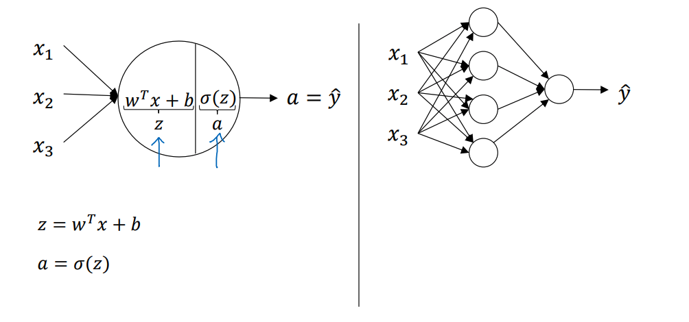


其中$x_{1},x_{2},x_{3}$代表的是样本的特征，这里用向量这矩阵来形象的解释(主要是为了不使用for)
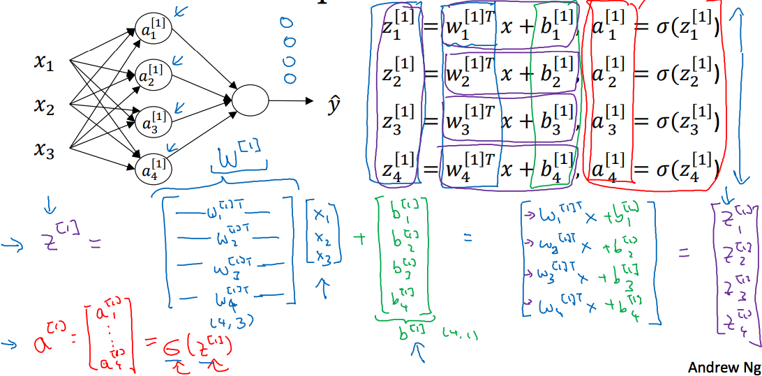
以单样本为例：

$$z_{1}^{[1]}=\begin{bmatrix} w_{11}^{[1]}\\ w_{12}^{[1]} \\ w_{13}^{[1]} \end{bmatrix}^{T}\begin{bmatrix} x_{1}\\ x_{2} \\ x_{3} \end{bmatrix}+ b_{1}^{[1]}\,\,\,\, ,\,\,\,\,z_{2}^{[1]}=\begin{bmatrix} w_{21}^{[1]}\\ w_{22}^{[1]} \\ w_{23}^{[1]} \end{bmatrix}^{T}\begin{bmatrix} x_{1}\\ x_{2} \\ x_{3} \end{bmatrix}+ b_{2}^{[1]}\,\,\,...$$

w矩阵行表示该层神经元个数，列表示样本特征个数，b向量长度为该层神经元的个数，即$w^{[1]}.shape=(4,3)，z^{[1]}.shape=(4,1)，w^{[2]}.shape=(1,3)，z^{[2]}.shape=(1,1)$可表示为：

$$w^{[1]}=\begin{bmatrix} w_{11}^{[1]}& w_{12}^{[1]} & w_{13}^{[1]}\\ w_{21}^{[1]}& w_{22}^{[1]} & w_{23}^{[1]}\\ w_{31}^{[1]}& w_{32}^{[1]} & w_{33}^{[1]}\\ w_{41}^{[1]}& w_{42}^{[1]} & w_{43}^{[1]}\\ \end{bmatrix}\\ z^{[1]}=w^{[1]}\begin{bmatrix} x_{1}\\ x_{2} \\ x_{3} \end{bmatrix}+\begin{bmatrix} b_{1}^{[1]}\\ b_{2}^{[1]} \\ b_{3}^{[1]}\\b_{4}^{[1]} \end{bmatrix}\\ a^{[1]}=\sigma(z^{[1]})\\ z^{[2]}=w^{[2]}a^{[1]}+b^{[2]}=\begin{bmatrix} w_{21}^{[2]}& w_{22}^{[2]} & w_{23}^{[2]} \end{bmatrix}a^{[1]}+b^{[2]}$$

3.4 Vectorizing across multiple examples

那么对于多个样本，同样是上面那个神经网络，用矩阵去掉下面这个for：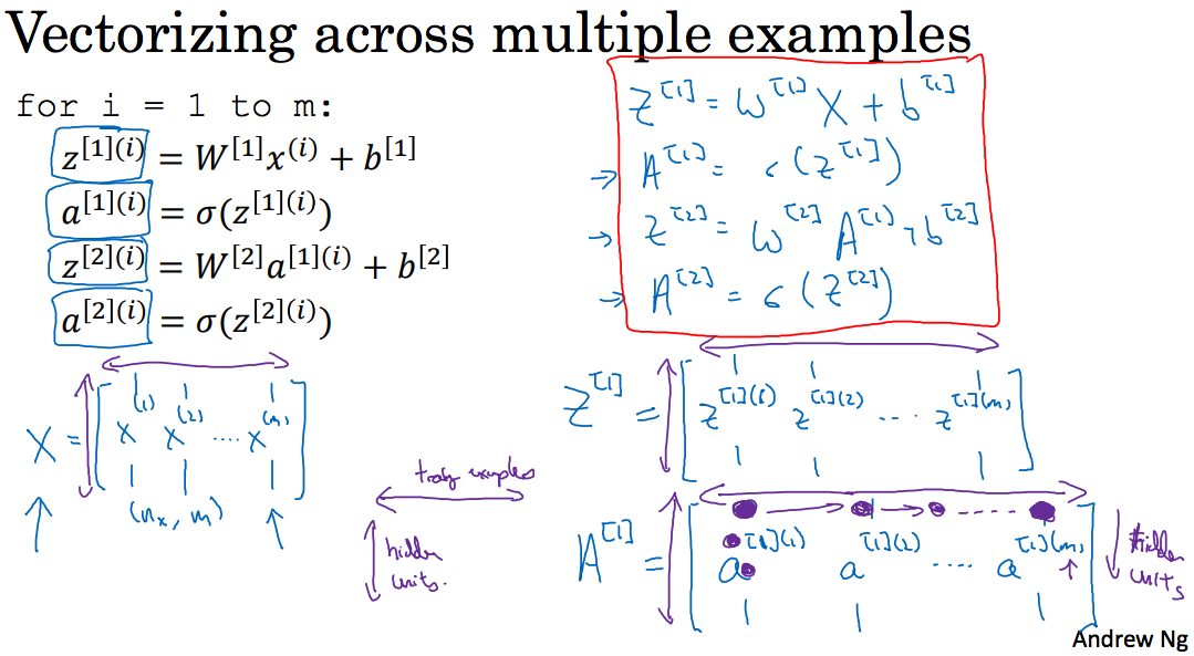

m为样本个数，X矩阵(行为样本个数，列为样本特征个数)，$Z^{[1]}.shape=(4,m)$，$Z^{[2]}.shape=(1,m)$，如下：

$$X=\begin{bmatrix} x_{1}^{(1)}&x_{1}^{(2)} &...& x_{1}^{(m)}\\ x_{2}^{(1)}& x_{2}^{(2)} &...& x_{2}^{(m)}\\ x_{3}^{(1)}& x_{3}^{(2)} &...&x_{3}^{(m)} \end{bmatrix}\\ Z^{[1]}=\begin{bmatrix} w_{11}^{[1]}& w_{12}^{[1]} & w_{13}^{[1]}\\ w_{21}^{[1]}& w_{22}^{[1]} & w_{23}^{[1]}\\ w_{31}^{[1]}& w_{32}^{[1]} & w_{33}^{[1]}\\ w_{41}^{[1]}& w_{42}^{[1]} & w_{43}^{[1]}\\ \end{bmatrix}X+\begin{bmatrix} b_{1}^{[1]}&...&b_{1}^{[1]}\\ b_{2}^{[1]}&...& b_{2}^{[1]} \\ b_{3}^{[1]}&...&b_{3}^{[1]} \\b_{4}^{[1]}&...&b_{3}^{[1]} \end{bmatrix}\\ A^{[1]}=\sigma(Z^{[1]})\\ Z^{[2]}=W^{[2]}A^{[1]}+b^{[2]}=\begin{bmatrix} w_{21}^{[2]}& w_{22}^{[2]} & w_{23}^{[2]}\\ \end{bmatrix}A^{[1]}+\begin{bmatrix} b^{[2]}& ...&b^{[2]} \\ \end{bmatrix}\\ A^{[2]}=\sigma(Z^{[2]})$$

3.6 Activation functions

讲到了sigmoid，tanh，Relu，leaky Relu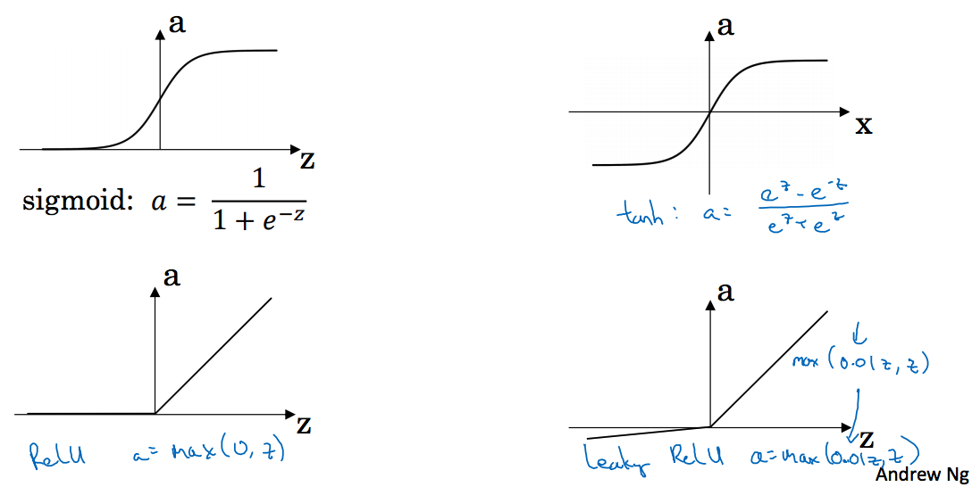

这里以这几个问题简单的讲解一下激活函数：为什么要使用激活函数，激活函数有哪些性质，各个激活函数有什么区别？

对于简单的样本分类可以使用线性拟合，但是对于复杂的样本，线性不可分的情况就需要引入非线性函数，也就是说对于神经网络中如果直接令$a=z$的话，组合起来永远都是线性的，根本不需要多层网络；

激活函数被定义为处处可微的函数，几个概念，关于饱和，硬饱和，软饱和
饱和：当激活函数h(x)满足

$$\lim_{n \to +\infty} h'(x)=0$$

称为右饱和
当激活函数h(x)满足

$$\lim_{n \to -\infty} h'(x)=0$$

称为左饱和
硬饱和：对任意的x，如果存在常数c，当x>c时恒有 h′(x)=0则称其为右硬饱和，反之左硬饱和
软饱和：如果只有在极限状态下偏导数等于0的函数，称之为软饱和

Sigmoid函数
输出映射到(0，1)之间，可作为输出层，但是由于软饱和性，容易产生梯度消失，最终导致信息丢失，从而无法完成深层网络训练；而且反向传播求解梯度时涉及除法，计算量大；其输出不是以0为中心。[3点]

此处讲一下梯度消失是什么，为什么梯度消失就会导致信息丢失？
梯度消失就是当sigmoid非常接近0，1时，对应的梯度会非常的小，而如果神经网络的层数又非常大的话，由于梯度的最大值是1/4，反向传播导致连乘导致前面层的梯度会越来越小，近乎与随机，这样就起不到训练的效果，即信息丢失。

再讲一下Sigmoid输出不是zero-centered，而下面的tanh是zero-centered？
网上说的感觉有问题，也没看太明白，说Sigmoid在梯度下降时如果输入x全为正或者负，会导致下降缓慢，而tanh就不会，后面又说批量导入数据的话可以解决，我没太明白zero-centered，ng说使用tanh激活函数的平均值接近于0，当你训练数据的时候，可能需要平移所有数据，让数据平均值为0，使用tanh而不是Sigmoid函数，可以达到让数据中心化的效果，上层的结果接近于0而不是0.5，实际上让下一层的学习更方便[会在第二门课中详细讨论]
下面这段似乎更清楚了：
Sigmoid outputs are not zero-centered result, in later layers of processing this would be receiving data that is not zero-centered. This has implications because if the data coming into a neuron is always positive, then the gradient on the weights w will during backpropagation become either all be positive, or all negative. This could introduce undesirable zig-zagging dynamics in the gradient updates for the weights, and that will be inconvenience.
参考：Why would we want neuron outputs to be zero centered in neural networks?

tanh函数
比Sigmoid函数收敛速度更快，和Sigmoid相比输出是以0为中心，同样由于软饱和性会产生梯度消失。

ReLU函数
相比于Sigmoid和tanh，ReLU在SGD中能够快速收敛，运算简单，缓解了梯度消失的问题，提供了神经网络的稀疏表达能力；但是随着训练的进行，神经元会出现死亡，权重无法更新，即从该时刻起，神经元输出将永远是0【不幸的初始化，或者learning rate太高】
其输出不是zero-centered
ReLU目前仍然是最常用的activation function

Leaky ReLU函数

$$f(x)=max(0.01x,x)$$

为了解决ReLU的Dead ReLU Problem，提出ReLU的前半段设置为0.01x而不是0，在实际操作中并没有完全证明Leaky ReLU总是好于ReLU的

softmax函数
用于多分类神经网络的输出

$$\sigma(z)_{j}=\frac{e^{z_j}}{\sum_{k=1}^{K}e^{z_k}}$$

如上公式，表明那个$z_{j}$大于其它的$z_{i}$，那么这个分量就逼近于1，然后选取最大的那个作为输出，这里选择指数是因为要让大的更大，并且需要函数可导。
参考
CS231N-Lecture5 Training Neural Network
聊一聊深度学习的activation function
深度学习中的激活函数与梯度消失
浅谈深度学习中的激活函数

3.9 Gradient descent for neural networks

继续上图，仍旧以前面的神经网络为例，前面讲到正向传播过程，此处是反向传播过程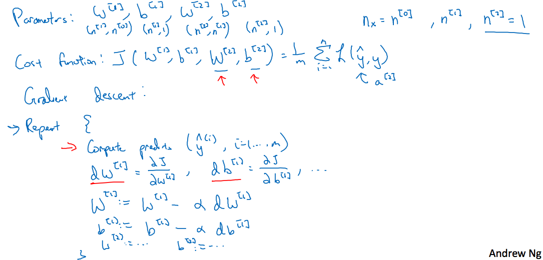


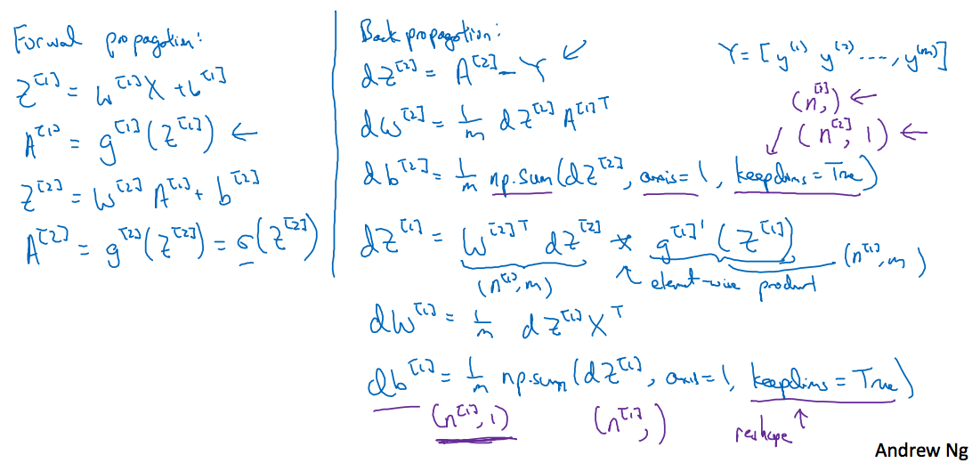
讲的很清楚了，这里$n^{[i]}$表示的是第i层的神经元个数，这样对应的各参数维度有

$$w^{[1]}.shape=(n^{[1]},b^{[0]})，b^{[1]}.shape=(n^{[1]},1)，\\w^{[2]}.shape=(n^{[2]},n^{[1]})，b^{[2]}.shape=(n^{[2]},1)$$

关于求解梯度，可以参考第二周的详细笔记，这里仅对$dZ^{[1]}$解释(视频中讲到第二层的激活函数使用Sigmoid函数，第一层的激活函数设置为g(x)，与前面前向传播中都使用Sigmoid函数的不同，一般来说对于二分类最后一层使用Sigmoid函数，而其它层应该尽量避免使用Sigmoid函数)

$$dZ^{[1]}=\frac{dJ}{dZ^{[1]}}=\frac{dJ}{dA^{[2]}} \cdot \frac{dA^{[2]}}{dZ^{[2]}}\cdot \frac{dZ^{[2]}}{dA^{[1]}}\cdot \frac{dA^{[1]}}{dg(Z^{[1]})}\cdot\frac{dg(Z^{[1]})}{dZ^{[1]}}\\ =(W^{[2]})^{T}dZ^{[2]}\cdot g'^{[1]}(Z^{[1]})$$

这里dz和z的维度相同，因此在计算梯度的过程中注意维度
下面是自己用python实现仅含有一层隐含层的神经网络前向反向传播算法，激活函数均为Sigmoid函数

import numpy as np


def sigmoid(z):
    s = 1 / (1 + np.exp(-z))
    return s
    
"""
X为n行（特征）m列（样本个数）
Y为1行m列（样本标签）
n1为神经网络的第一层神经元的个数（隐藏层，不算输入层），这里是3
n2为输出层的神经元个数，这里是1
"""
def forward_backward_code(X,Y,n1,n2,num_iter,learning_rate):
    n,m=X.shape
    #参数初始化
    W1=np.random.randn(n1,n)
    b1=np.zeros((n1,1))
    W2=np.random.randn(n2,n1)
    b2=np.zeros((n2,1))
    for i in num_iter:
        #前向传播
        Z1=np.dot(W1,X)+b1
        A1=sigmoid(Z1)
        Z2=np.dot(W2,A1)+b2
        A2=sigmoid(Z2)
        #反向传播
        dZ2=A2-Y
        dW2=1/m*np.dot(dZ2,A1.T)
        db2=1/m*np.sum(dZ2,axis=1,keepdims=True)
        dZ1=np.dot(W2.T,dZ2)*sigmoid(Z1)(1-sigmoid(Z1))
        dW1=1/m*np.dot(dZ1,X.T)
        db1=1/m*np.sum(dZ1,axis=1,keepdims=True)
        #更新参数
        W2=W2-learning_rate*dW2
        b2=b2-learning_rate*db2
        W1=W1-learning_rate*dW1
        b1=b1-learning_rate*db1

虽然照着公式写出了代码，但是这里我还是想详细的讲述一下该神经网络反向求导的过程
见第4周，用维度来讲解，不过如果要想搞清楚其中原理还是使用纯变量来计算最后再转化为矩阵看效果，不过这样得不偿失！

最后讲到了初始化的问题，为什么不能全部初始化为0，这里原因是因为如果全部初始化为0后，导致输出的结果一样，而且在反向传播的过程中每层的dw会一样，导致每层w相同，无法拟合模型

大作业

地址：Planar data classification with one hidden layer v4
其中planar_utils文件请参考deep-learning-specialization-coursera

数据集X维度为(2，400)，Y的维度为(1，400)，这里先使用sklearn中的logistic回归来拟合

import numpy as np
import matplotlib.pyplot as plt
import sklearn.linear_model
from planar_utils import plot_decision_boundary, sigmoid, load_planar_dataset, load_extra_datasets

X, Y = load_planar_dataset()
clf = sklearn.linear_model.LogisticRegressionCV();
clf.fit(X.T, Y.T);
# Plot the decision boundary for logistic regression
plot_decision_boundaryLR_predictions = clf.predict(X.T)
print ('Accuracy of logistic regression: %d ' % float((np.dot(Y,LR_predictions) + np.dot(1-Y,1-LR_predictions))/float(Y.size)*100) +
       '% ' + "(percentage of correctly labelled datapoints)")(lambda x: clf.predict(x), X, Y)
plt.title("Logistic Regression")
LR_predictions = clf.predict(X.T)
print ('Accuracy of logistic regression: %d ' % float((np.dot(Y,LR_predictions) + np.dot(1-Y,1-LR_predictions))/float(Y.size)*100) +
       '% ' + "(percentage of correctly labelled datapoints)")

输出如下：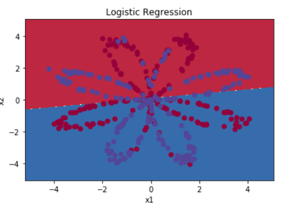

Accuracy of logistic regression: 47 % (percentage of correctly labelled datapoints)

显然logistic回归在非线性数据的分类上效果很差，下面用含一个隐藏层的神经网络来实现该数据集上的分类，下面是函数代码及解释过程，更详细的说明请参考原文

初始化参数
Instructions:

• Make sure your parameters’ sizes are right. Refer to the neural network figure above if needed.
• You will initialize the weights matrices with random values.
  Use: np.random.randn(a,b) * 0.01 to randomly initialize a matrix of shape (a,b).
• You will initialize the bias vectors as zeros.
  Use: np.zeros((a,b)) to initialize a matrix of shape (a,b) with zeros.

def initialize_parameters(n_x, n_h, n_y):
    """
    Argument:
    n_x -- size of the input layer
    n_h -- size of the hidden layer
    n_y -- size of the output layer
    
    Returns:
    params -- python dictionary containing your parameters:
                    W1 -- weight matrix of shape (n_h, n_x)
                    b1 -- bias vector of shape (n_h, 1)
                    W2 -- weight matrix of shape (n_y, n_h)
                    b2 -- bias vector of shape (n_y, 1)
    """
    np.random.seed(2) # we set up a seed so that your output matches ours although the initialization is random.
    W1 = np.random.randn(n_h,n_x)*0.01
    b1 = np.zeros((n_h,1))
    W2 = np.random.randn(n_y,n_h)*0.01
    b2 = np.zeros((n_y,1))
    assert (W1.shape == (n_h, n_x))
    assert (b1.shape == (n_h, 1))
    assert (W2.shape == (n_y, n_h))
    assert (b2.shape == (n_y, 1))
    parameters = {"W1": W1,
                  "b1": b1,
                  "W2": W2,
                  "b2": b2}
    return parameters

前向传播

def forward_propagation(X, parameters):
    """
    Argument:
    X -- input data of size (n_x, m)
    parameters -- python dictionary containing your parameters (output of initialization function)
    
    Returns:
    A2 -- The sigmoid output of the second activation
    cache -- a dictionary containing "Z1", "A1", "Z2" and "A2"
    """
    W1 = parameters['W1']
    b1 = parameters['b1']
    W2 = parameters['W2']
    b2 = parameters['b2']
 
    Z1 = np.dot(W1,X)+b1
    A1 = np.tanh(Z1)
    Z2 = np.dot(W2,A1)+b2
    A2 = sigmoid(Z2)
    
    assert(A2.shape == (1, X.shape[1]))
    
    cache = {"Z1": Z1,
             "A1": A1,
             "Z2": Z2,
             "A2": A2}
    return A2, cache

成本函数
Instructions:

• There are many ways to implement the cross-entropy loss. To help you, we give you how we would have implemented $−\sum_{i=0}^{m}y(i)log(a^{[2](i)})$ :
  logprobs = np.multiply(np.log(A2),Y)
  cost = - np.sum(logprobs) # no need to use a for loop!

(you can use either np.multiply() and then np.sum() or directly np.dot()).

def compute_cost(A2, Y, parameters):
    """
    Computes the cross-entropy cost given in equation (13)
    
    Arguments:
    A2 -- The sigmoid output of the second activation, of shape (1, number of examples)
    Y -- "true" labels vector of shape (1, number of examples)
    parameters -- python dictionary containing your parameters W1, b1, W2 and b2
    
    Returns:
    cost -- cross-entropy cost given equation (13)
    """
    m = Y.shape[1] # number of example

    logprobs = np.multiply(np.log(A2),Y)+ np.multiply((1-Y), np.log(1-A2))
    cost = -1/m*np.sum(logprobs)
    
    cost = np.squeeze(cost)     # makes sure cost is the dimension we expect. 
                                # E.g., turns [[17]] into 17 
    assert(isinstance(cost, float))
    
    return cost

反向传播函数
Tips:

• To compute dZ1 you’ll need to compute $g^{[1]′}(Z^{[1]})$. Since $g^{[1]}(.)$ is the tanh activation function, if $a=g^{[1]}(z)$then $g^{[1]′}(z)=1−a^2$ . So you can compute $g^{[1]′}(Z^{[1]})$using (1 - np.power(A1, 2)).

def backward_propagation(parameters, cache, X, Y):
    """
    Implement the backward propagation using the instructions above.
    
    Arguments:
    parameters -- python dictionary containing our parameters 
    cache -- a dictionary containing "Z1", "A1", "Z2" and "A2".
    X -- input data of shape (2, number of examples)
    Y -- "true" labels vector of shape (1, number of examples)
    
    Returns:
    grads -- python dictionary containing your gradients with respect to different parameters
    """
    m = X.shape[1]
    
    # First, retrieve W1 and W2 from the dictionary "parameters".
    W1 = parameters['W1']
    W2 = parameters['W2']
        
    # Retrieve also A1 and A2 from dictionary "cache".
    A1 = cache['A1']
    A2 = cache['A2']
    
    # Backward propagation: calculate dW1, db1, dW2, db2. 
    dZ2 = A2-Y
    dW2 = 1/m*np.dot(dZ2,A1.T)
    db2 = 1/m*np.sum(dZ2,axis=1,keepdims=True)
    dZ1 = np.multiply(np.dot(W2.T,dZ2),1-np.power(A1,2))
    dW1 = 1/m*np.dot(dZ1,X.T)
    db1 = 1/m*np.sum(dZ1,axis=1,keepdims=True)
    
    grads = {"dW1": dW1,
             "db1": db1,
             "dW2": dW2,
             "db2": db2}
    
    return grads

参数更新
给出两张图，对应着learning_rate
The gradient descent algorithm with a good learning rate (converging) and a bad learning rate (diverging). Images courtesy of Adam Harley

def update_parameters(parameters, grads, learning_rate = 1.2):
    """
    Updates parameters using the gradient descent update rule given above
    
    Arguments:
    parameters -- python dictionary containing your parameters 
    grads -- python dictionary containing your gradients 
    
    Returns:
    parameters -- python dictionary containing your updated parameters 
    """
    # Retrieve each parameter from the dictionary "parameters"
    W1 = parameters['W1']
    b1 = parameters['b1']
    W2 = parameters['W2']
    b2 = parameters['b2']
    # Retrieve each gradient from the dictionary "grads"
    dW1 = grads['dW1']
    db1 = grads['db1']
    dW2 = grads['dW2']
    db2 = grads['db2']
    # Update rule for each parameter
    W1 = W1-learning_rate*dW1
    b1 = b1-learning_rate*db1
    W2 = W2-learning_rate*dW2
    b2 = b2-learning_rate*db2
    
    parameters = {"W1": W1,
                  "b1": b1,
                  "W2": W2,
                  "b2": b2}
    
    return parameters

模型训练

def nn_model(X, Y, n_h, num_iterations = 10000, print_cost=False):
    """
    Arguments:
    X -- dataset of shape (2, number of examples)
    Y -- labels of shape (1, number of examples)
    n_h -- size of the hidden layer
    num_iterations -- Number of iterations in gradient descent loop
    print_cost -- if True, print the cost every 1000 iterations
    
    Returns:
    parameters -- parameters learnt by the model. They can then be used to predict.
    """
    
    np.random.seed(3)
    n_x = layer_sizes(X, Y)[0]
    n_y = layer_sizes(X, Y)[2]
    
    # Initialize parameters, then retrieve W1, b1, W2, b2. Inputs: "n_x, n_h, n_y". Outputs = "W1, b1, W2, b2, parameters".
    parameters = initialize_parameters(n_x,n_h,n_y)
    W1 = parameters['W1']
    b1 = parameters['b1']
    W2 = parameters['W2']
    b2 = parameters['b2']
    # Loop (gradient descent)

    for i in range(0, num_iterations):
         
        A2, cache = forward_propagation(X, parameters)
        # Cost function. Inputs: "A2, Y, parameters". Outputs: "cost".
        cost = compute_cost(A2, Y, parameters)
        # Backpropagation. Inputs: "parameters, cache, X, Y". Outputs: "grads".
        grads = backward_propagation(parameters, cache, X, Y)
        # Gradient descent parameter update. Inputs: "parameters, grads". Outputs: "parameters".
        parameters = update_parameters(parameters, grads, learning_rate = 1.2)
        # Print the cost every 1000 iterations
        if print_cost and i % 1000 == 0:
            print ("Cost after iteration %i: %f" %(i, cost))

    return parameters

模型预测
As an example, if you would like to set the entries of a matrix X to 0 and 1 based on a threshold you would do: X_new = (X > threshold)
比如下面的Sigmoid输出后，要求其值大于0.5的输出1，否则输出0

def predict(parameters, X):
    """
    Using the learned parameters, predicts a class for each example in X
    
    Arguments:
    parameters -- python dictionary containing your parameters 
    X -- input data of size (n_x, m)
    
    Returns
    predictions -- vector of predictions of our model (red: 0 / blue: 1)
    """
    
    # Computes probabilities using forward propagation, and classifies to 0/1 using 0.5 as the threshold.
    A2, cache = forward_propagation(X, parameters)
    predictions = (A2>0.5)
    return predictions

训练+预测+结果

# Build a model with a n_h-dimensional hidden layer
parameters = nn_model(X, Y, n_h = 4, num_iterations = 10000, print_cost=True)

# Plot the decision boundary
plot_decision_boundary(lambda x: predict(parameters, x.T), X, Y)
plt.title("Decision Boundary for hidden layer size " + str(4))

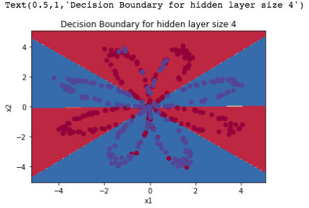
Accuracy: 90%

继续做了一个测试，来看隐藏层神经元的个数对神经网络训练的影响，这里就不放图片了

plt.figure(figsize=(16, 32))
hidden_layer_sizes = [1, 2, 3, 4, 5, 20, 50]
for i, n_h in enumerate(hidden_layer_sizes):
    plt.subplot(5, 2, i+1)
    plt.title('Hidden Layer of size %d' % n_h)
    parameters = nn_model(X, Y, n_h, num_iterations = 5000)
    plot_decision_boundary(lambda x: predict(parameters, x.T), X, Y)
    predictions = predict(parameters, X)
    accuracy = float((np.dot(Y,predictions.T) + np.dot(1-Y,1-predictions.T))/float(Y.size)*100)
    print ("Accuracy for {} hidden units: {} %".format(n_h, accuracy))

Accuracy for 1 hidden units: 67.5 %
Accuracy for 2 hidden units: 67.25 %
Accuracy for 3 hidden units: 90.75 %
Accuracy for 4 hidden units: 90.5 %
Accuracy for 5 hidden units: 91.25 %
Accuracy for 20 hidden units: 90.5 %
Accuracy for 50 hidden units: 90.75 %