神经网络和深度学习[1-2]
神经网络和深度学习[1-3]
神经网络和深度学习[1-4]
改善深层神经网络:超参数调试、正则化以及优化【2-1】
改善深层神经网络:超参数调试、正则化以及优化【2-2】
改善深层神经网络:超参数调试、正则化以及优化【2-3】
结构化机器学习项目 3
2.3 logistic Regression: Cost Function
二分类问题,每个特征前面有一个权重,然后加上一个偏置项,即,我们想让这个结果要么是0,要么是1,那么就用到了sigmod函数,即,讲义中给出的是对于样本而言,有如下公式:
该样本的损失函数(loss function)一般为,但是在logistic回归中一般使用下面的损失函数:
原因是因为平方损失函数(误差平方)在讨论最优化问题的时候是非凸的,即会得到多个局部最优解(梯度下降法可能找不到全局最优解),而用log损失函数,起着和误差平方相似的作用,会给我们一个凸的优化问题,很容易做优化。
对于多个样本的成本函数(cost function) J 如下:
成本函数是损失函数的平均值,通过改变参数w,b来使成本函数最小
【补充】:这节课有几个地方需要补充:为什么log损失是凸的,为什么误差平方使用梯度可能找不到全局最优,损失函数有哪几种,该如何使用
log的损失函数标准形式是:,和上面的对应的
先给出logistic回归针对二分类的模型表达式:
这样对应上面的损失函数,就会得到成本函数【注意:损失函数衡量单个样本,成本函数衡量多个样本】:
而log函数是单调递增的,所以logP(Y|X)也是单调递增的,而-logP(Y|X)即为单调递减,这样使用梯度下降就可以找到全局最小值
而误差平方函数本身就是二次曲线,虽然是凸的,但是组合成的成本函数就不是凸的了
关于损失函数,这里只简单的提一下:
给出这么几种损失函数:
Among all linear methods , we need to first determine the form of , and then finding by formulating it to maximizing likelihood or minimizing loss. This is straightforward.
For classification, it’s easy to see that if we classify correctly we have , and if incorrectly. Then we formulate following loss functions:
- 0/1 loss: . We define if , and o.w. Non convex and very hard to optimize.
- Hinge loss: approximate 0/1 loss by . We define . Apparently is small if we classify correctly.
- Logistic loss: . Refer to my logistic regression notes for details.
For regression:
- Square loss:
Fortunately, hinge loss, logistic loss and square loss are all convex functions. Convexity ensures global minimum and it’s computationally appleaing.
参考:http://www.cs.cmu.edu/~yandongl/loss.html
继续来看这些函数直观的意义,均匀取-2到2之间的点作为误差值,针对不同的损失函数,采取不同的处理方式,如下:
如下图: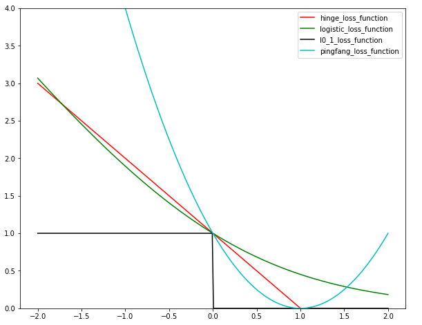
上面这个图需要明白一点,x轴代表的是上面提到的,我们希望达到的目标是该值越大(正值)越好,也就是越远离0,这样我们的模型f就越好,因为这样拟合会很好(可以这样理解:对于坐标上的两种类型的点,我们找到一条直线将其分隔开,这条直线应该是离各类型的点最远的线,虽然靠近某一类型的点来划分也可以,但是这样预测能力就会降低)
其中可以看到0/1损失函数是最理想的,只要误差小于0,结果就是1;hinge损失函数是当误差小于1结果才为0,也就是说要求就好;而log损失函数就是要求越大越好;其中平方损失函数这个是不适合分类的,如果用分类的化,必须取的结果来作为损失函数(感知机就是这样)。
关于使用方面:二分类问题一般使用log损失或者是Hinge损失函数,回归问题一般使用平方损失函数。
2.4 Gradient Descent
关于梯度下降,这里放一张图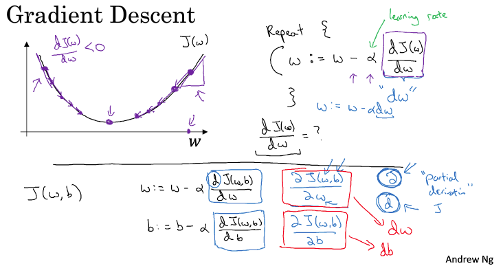
如上图,就以为例,我们现在要找到使J最小的w,对于给定的,我们需要找到最小的J,变量的更新应该是沿着梯度方向,更新w:
如果在左边,就增加w;如果在右边,就减小w
2.10 Logistic regression on m examples
这里将2.9节讲到的logistic回归中的梯度下降和对m个样例的梯度下降结合起来,并用python实现最原始的代码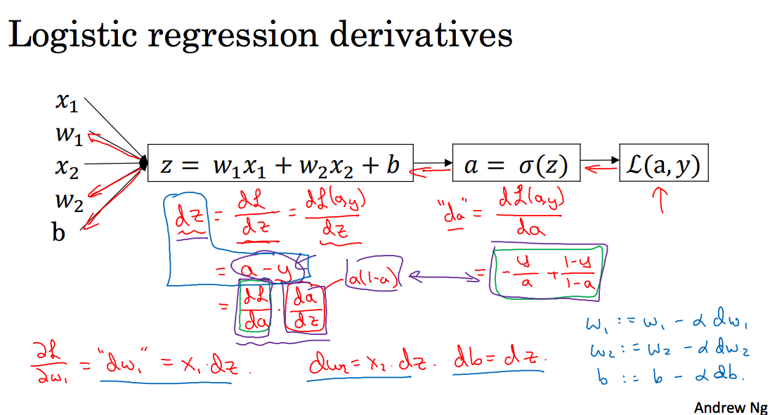
上图其实在讲反向传播算法,而且讲到了反向传播算法中的最原始的计算方式
这里对其中的每一个变量求导(遵循视频中的讲解,使用da代表损失函数对a的求导):
其中对于Sigmoid的求导公式
更新:
上面是对单个样本的梯度更新,下面logistic回归在多个样本上的python代码实现【理解此部分代码对于理解这两节讲的内容我觉得很重要,该代码为自己编写,可能存在错误】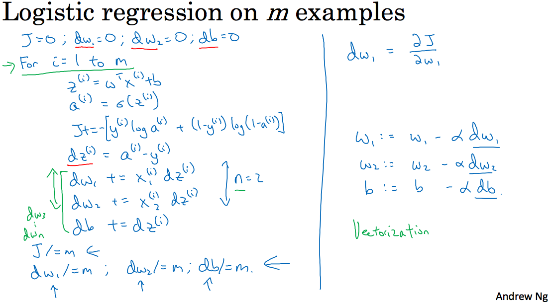
2.11 Vectorization
这节讲要避免使用for,而使用向量,这里举了一个例子,是使用np.dot来计算向量和for运算时间的对比:
Vectorized version:1.27410888671875ms
for version:702.2850513458252ms
2.12 More vectorization examples
这一节讲到之前的logistic回归的代码可以使用向量优化,做一下修改,简化了一重循环,如下:
2.14 Vectorizing Logistic Regression’s Gradient Computation
这两节在讲简化上面的代码,如下图所示: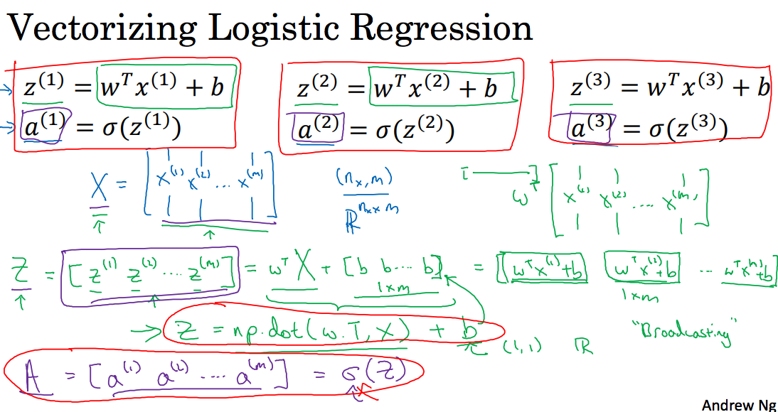
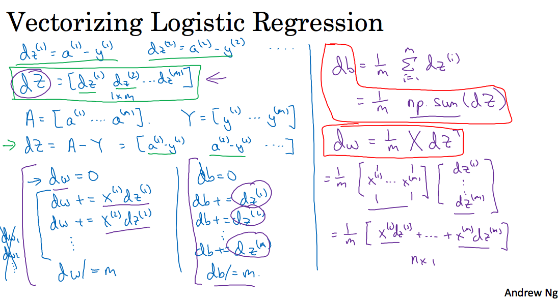
代码如下:
Broadcasting in Python
如下图,对于向量和数值(scaler)运算,scaler会自动补齐对应的行/列;同样的道理,矩阵和向量的运行,向量也会相应的补齐对应的行/列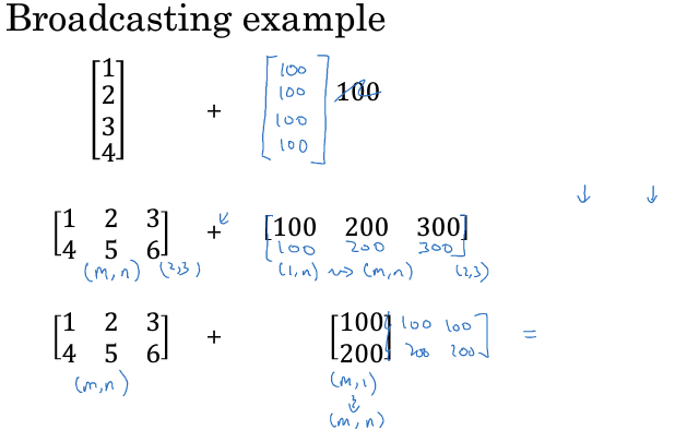
大作业
这个作业基本上前面基本上已经实践过了,作业地址:Logistic Regression with a Neural Network mindset v4
1 - packgeds
首先是导入数据,这句from lr_utils import load_dataset,我的jupter中没有lr_utils,就直接将lr_utils.py和对应的datasets集拷贝过来了github
2 - Overview of the Problem set
|
|
Exercise: Reshape the training and test data sets so that images of size (num_px, num_px, 3) are flattened into single vectors of shape (num_px ∗∗ num_px ∗∗ 3, 1).
A trick when you want to flatten a matrix X of shape (a,b,c,d) to a matrix X_flatten of shape (b ∗∗ c ∗∗ d, a) is to use:
X_flatten = X.reshape(X.shape[0], -1).T # X.T is the transpose of X
train_set_x_flatten shape: (12288, 209)
train_set_y shape: (1, 209)
test_set_x_flatten shape: (12288, 50)
test_set_y shape: (1, 50)
sanity check after reshaping: [17 31 56 22 33]
One common preprocessing step in machine learning is to center and standardize your dataset, meaning that you substract the mean of the whole numpy array from each example, and then divide each example by the standard deviation of the whole numpy array. But for picture datasets, it is simpler and more convenient and works almost as well to just divide every row of the dataset by 255 (the maximum value of a pixel channel).
Let’s standardize our dataset.
4 - General Architecture of the learning algorithm
省略了3
Exercise: Using your code from “Python Basics”, implement sigmoid(). As you’ve seen in the figure above, you need to compute to make predictions. Use np.exp()
Initializing parameters
Forward and Backward propagation
Exercise: Implement a function propagate() that computes the cost function and its gradient.
Hints:
Forward Propagation:
You get X
You compute
You calculate the cost function:
Here are the two formulas you will be using:
|
|
Exercise: Write down the optimization function. The goal is to learn ww and bb by minimizing the cost function J . For a parameter θ, the update rule is θ=θ−α dθ , where α is the learning rate.
Exercise: The previous function will output the learned w and b. We are able to use w and b to predict the labels for a dataset X. Implement the predict() function. There is two steps to computing predictions:
- Calculate
- Convert the entries of a into 0 (if activation <= 0.5) or 1 (if activation > 0.5), stores the predictions in a vector Y_prediction. If you wish, you can use an if/else statement in a for loop (though there is also a way to vectorize this).1234567891011121314151617181920212223242526272829303132def predict(w, b, X):'''Predict whether the label is 0 or 1 using learned logistic regression parameters (w, b)Arguments:w -- weights, a numpy array of size (num_px * num_px * 3, 1)b -- bias, a scalarX -- data of size (num_px * num_px * 3, number of examples)Returns:Y_prediction -- a numpy array (vector) containing all predictions (0/1) for the examples in X'''m = X.shape[1]Y_prediction = np.zeros((1,m))w = w.reshape(X.shape[0], 1)# Compute vector "A" predicting the probabilities of a cat being present in the picture### START CODE HERE ### (≈ 1 line of code)A = sigmoid(np.dot(w.T,X)+b)### END CODE HERE ###for i in range(A.shape[1]):# Convert probabilities A[0,i] to actual predictions p[0,i]### START CODE HERE ### (≈ 4 lines of code)if A[0][i]>0.5:Y_prediction[0][i]=1### END CODE HERE ###assert(Y_prediction.shape == (1, m))return Y_prediction
5 -Merge all functions into a model
You will now see how the overall model is structured by putting together all the building blocks (functions implemented in the previous parts) together, in the right order.
Exercise: Implement the model function. Use the following notation:
- Y_prediction for your predictions on the test set
- Y_prediction_train for your predictions on the train set
- w, costs, grads for the outputs of optimize()
|
|
|
|
train accuracy: 99.04306220095694 %
test accuracy: 70.0 %
到此就结束了,当然我们用训练集拟合,再对训练集预测,准确度肯定接近于1了,而测试集上只有70,说明过拟合了(我们的目的是让训练集和测试集结果尽量相同)
我这里按照教程将迭代次数改为5000后的结果:
learning rate is: 0.01
train accuracy: 100.0
test accuracy: 68.0
learning rate is: 0.001
train accuracy: 96.65071770334929
test accuracy: 74.0
learning rate is: 0.0001
train accuracy: 77.51196172248804
test accuracy: 56.0
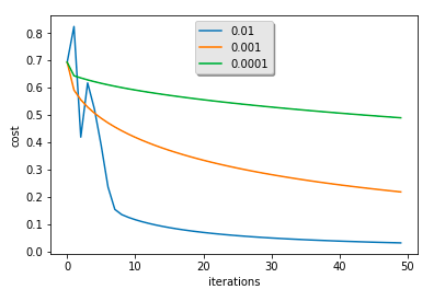
这里可以看到如果学习率为0.001时,在测试集上的结果达到了74,这是因为由于学习率比较小,也就是沿梯度下降慢(从图中也可以很明显的发现),训练集并没有完全收敛,那么就谈不上过拟合,也就是说如果迭代次数继续加大,在0.001上仍然可以找到更好的结果,同理对0.1而言,减小迭代次数也可以发现更好的结果;不过这些后没有必要,使用正则化或者其他可以解决过拟合问题
完!